The So-Called "Proof" of the Shell Theorem

The So-Called "Proof" of the Shell Theorem


Here is the typical "proof" for the Shell Theorem (the Hollow Sphere Theorem), as presented by university math faculties (this one was from saddleback.edu).

It was presented by a reader as "proof" that Newton was right about the force inside a uniform hollow sphere. (post #73) Of course the 'proof' does nothing of the kind.

As another reader (post #69) posted, a "theorem" in mathematical parlance is a mathematical statement considered to be "proven true" only in the sense that the mathematical result follows logically from the starting premises and the application of appropriate algebraic and rules and conventions. Even this idea of 'proven mathematically' isn't always clear, and theorems are constantly modified, limited, and expanded in the field of mathematics.

And a mathematical "proof" is not a in any sense a "physics" proof, which is based upon how well a given piece of mathematics actually applies to a physical situation, and its predictive power, when the mathematical variables and other elements are assigned to physical entities and measurements.

The so-called "proof" given begins by implicitly claiming to model a vague physical situation. None of the items below are properly defined, and none of the physical theory relating the idealized abstract model and its elements and diagram to a physical reality is ever presented or articulated. All of that remains not only unproven, but actually unstated. The premises and assumptions remain unexposed. Its appropriateness and accuracy of the theorem in encompassing a physical situation is left completely unexamined.


Essentially, the "proof" begins by ignoring the main physical problem. The author might have happily begun by explicitly making the admission:

"This 'proof' does not expound any physical theory. Nor does it examine the strength of the connection of its elements to physical realities. For that see a physics textbook. We are here only outlining a mathematical theorem:

Unlike our own diagram, nothing here is properly explained or labelled. None of the mathematical entities are described, and even key mathematical axioms and premises are left unacknowledged. For instance, the application of Sin and Cos functions have no meaning, even in mathematical proof, without the assumption of a Euclidean Spacetime manifold. But this is one of the very things to be proved in a gravity theory, and something that requires explicit discussion. We can't fault Newton for his ignorance of spacetime manifold options, but we can certainly fault a modern proponent of the "Shell Theorem" for failing to qualify his 'proofs' in the modern context.




Remarkably, a form of Newton's classic gravity equation simply appears in the third line here without any qualification or explanation. None of steps of the algebraic manipulation is shown, and none of the theorems or axioms required for these steps is given. No derivation or justification for any of the steps that are actually shown are explained.

We now have an equation, an integral, to which someone has assigned a physical meaning, by identifying the elements in the equation with elements in the original physical problem. While the substitution of variables and elements may be acceptable, the student/reader is left abandoned to the "God-like" presentation of the 'teacher'. The only hope is memorization of the forms acceptable on the exam, when the question is posed.

Now comes the hilarious part of the "proof":



"From the Tables:..." yes, that's right, the four difficult pages of real hardcore integration, and their theoretical underpinnings are skipped entirely, unlike our own appendix (see post #13) on the integration of this difficult integral (previous step). Naturally the 1st year student is not expected to know how to actually integrate a function like this. Like a trained monkey he must look it up in an advanced volume/table of Integrals, and simply jump to the next part of the problem.

This is not a formal 'proof' in fact of the Shell theorem or any other theorem. Its a "memorize" the entry in a table method, and don't ask any questions style of teaching suitable only for dummies.

Now, magically, the Force Vector F just appears. An algebraic equation has been derived (skipping all critical steps and techniques) for the force exerted on the object (not the sphere). No explanation for how the mathematics has been connected to a real physical vector is given. Essentially, all that has happened is that an equation from a book has been assigned a task.

A similar phoney implicit step has been performed for the Force vector in the separate case when the point-object is inside the shell/sphere. No notice of the failure of Newton's equation in the case where the particle is actually at the border of the shell is given. No explanation for what happens when a particle pierces the shell, exits/enters, is attempted.

The student is left with two equations, one of which reduces to a constant (0), but he has no idea of why there is no 'force' inside a 'uniform shell of insignificant thickness with its mass evenly distributed on its surface', or whether it is even true.

This is a classic example of the academic "bluster".

A bunch of algebra and some calculus references are waved in front of the inquirer, and they are just left feeling stupid, because in fact it is impossible to derive any proof of the Shell Theorem from this terse, highly condensed and deficient presentation of a complex operation which invokes literally hundreds of mathematical and physical assumptions.

The student is told to "go read the textbook discussion" on the Shell method of integration, or 'Newtonian Gravity'. He does the only thing possible in such a ridiculous situation: He memorizes the steps approved by the lecturer, gets his grade, and has no clue what is really transpiring in gravitational theory.

This is a classic example of what I would call the worst form of teaching imaginable, in spite of how common it is in institutions where bodies are pushed through the door and large amounts of money are collected.

Is the math incorrect?

 

What is disputed is a claim in a physical theory,
namely that the gravitational field inside any practical hollow sphere is zero,
either as a physical fact or as an approximation.

We are well aware of the mathematical apparatus and its 'value',
(for instance in the context of a developing algebraic Group),
but categorically reject any claim that any calculus operation can
intrinsically in any significant way 'prove' the validity of a physical theory.

Yet people as yourself keep focussing on whether or not the math is 'correct',
when the issue is actually,

"Does this cute mathematical artefact have any physical meaning?"

The question for a physicist will always be,

"Is this equation going to be accurate for my physical experiment,
in the manner in which I'm going to use it?",

not,

"Is this equation adequately defined as a mathematical entity,
to the satisfaction of esoteric mathematical theorists?"

As I already stated in post #65:

Quote:

This misunderstanding in regard to the purpose and meaning of Calculus, and indeed any mathematical result generally, i.e., its 'truth-content' in regard to reality, is one of the most common logical and epistemological errors in engineering, physics, and even amateur mathematics, and runs rampant in 'pop-science'.

(D) Failure of Sphere Theorem at Molecular Level

(D) Failure of Sphere Theorem at Molecular Level

CONTENTS
1. A Simple Quantization of Mass
2. General Method for Discrete Distributions of Mass
3. Discrete Form of Hollow Sphere Equation
4. Formula and Graph for Quantized Hollow Sphere
5. Sample Hollow Spheres of Discrete Particles
6. Summary and Conclusions with FAQs





1. A Simple Quantization of Mass
In a very general and straightforward sense, Newtonian gravity and electrostatics are already ‘quantized’ theories. That is, they begin and end with ‘corpuscles’ or ‘atoms’, discrete packets of finite, fixed mass and charge. These packets are viewed as concentrated point-masses or particles separated by relatively large amounts of empty space. This picture has turned out to be surprisingly accurate.







A salt crystal for instance is a regular cube-like pattern of atoms held in place by electromagnetic forces. Although rigid, it is actually mostly ‘space’, and its uniform density amounts to simply an even spacing in close-up view. While ‘regular’, the distribution of mass is not really and cannot ever be ‘uniform’. Instead, the mass ( or charge ) is ‘quantized’ spatially. We could say instead that the mass is uniformly distributed in discrete packets, equally spaced either throughout a volume or across an area.


Similarly, we can construct ‘hollow spheres’ at near-atom sizes by careful arrangement of atoms to form regular polyhedrons of various sizes and shapes.
A simple hollow sphere can be constructed out of carbon atoms for instance, with the required uniform spacing of atoms across the surface area, by placing the atoms at the vertexes of a dodecahedron.1 Although the synthesis of these exotic molecules is not easy, there is in principle no limit to the size or complexity possible of such spheres of ‘discrete uniform distribution of mass’. Naturally, one wants to know what the actual gravitational field for these objects is, both inside and out, and it turns out there is a straightforward method of calculating those forces.

_______________________
1. See Nazaroo’s article, A Fourth Isomer of Carbon , 1972

__________________




2. General Method for Discrete Distributions of Mass

Obviously for a handful of atoms one can simply calculate and sum the forces. For spheres larger than 20 times the size of an atom, where you have a hundred or more atoms distributed over a spherical surface, this is no longer practical. Yet we have not yet reached the size and quantity of particles required to treat the sphere as a smooth continuum of mass or charge spread over its surface.




Consider a sphere, of a size where about 20 atoms evenly spaced will reach around the circumference. As before, consider a test-mass, which we are going to move along the x-axis in a straight line through the centre and off again to infinity. At this size, the actual position of individual point-masses (charges) is not crucial, because our test-mass is not gettng that close to most of them.
Instead, we can construct an equivalent model of the sphere (as in the diagram) by placing rings equally spaced on the surface at about the same spacing as the original atoms. Along each ring we space equivalent atoms, again at the same spacing. The result will be an approximately even distribution of atoms at the desired resolution or spacing, which is all we really need. By inspection, we should be able to see that the overall sum of forces will not be affected by changing the actual latitudes of the individual rings, if we keep the spacing. We could have an even or odd number of rings, or slide the pattern across the surface like wallpaper, taking rings away at one end and adding them at the other.

At this point, the reader might ask, what if we can’t spread the atoms along a ring evenly at the required spacing? Suppose we need an extra half-atom to match up with our tail on some ring: No problem. From our previous analysis, we know that rings of evenly spread discrete points act just like continuous rings. That is, the y and z components cancel and we can simply use our ring formula. From the point of view of our test-mass, it makes no difference whether we have rings of discrete points or continuous rings. As long as we assign the correct total mass to each ring, we will calculate the correct force. We emphasize that this is does not compromise accuracy. It translates directly to the physical situation, at least as far as the force in the x direction is concerned.

In fact, using smooth rings will actually smooth out errors caused by our initial substitute model. It would have had some artificial ‘bumps’ since it isn’t possible to align rings with different numbers of point-masses properly. This isn’t the critical issue it appears, since plenty of polyhedral molecules might actually have such features.
It does matter that we assign the correct mass to each ring. The mass will naturally be based upon the number of particles. Since the particles are equally spaced all over the surface, each particle represents a fixed, equal amount of surface area, and hence particle number is also a measure of surface area. Since we have ‘unquantized’ the sphere in the y and z -direction by using smooth rings, we can now have non-integer values for ‘particle units’. These ‘particle units’ are interchangable with area units.


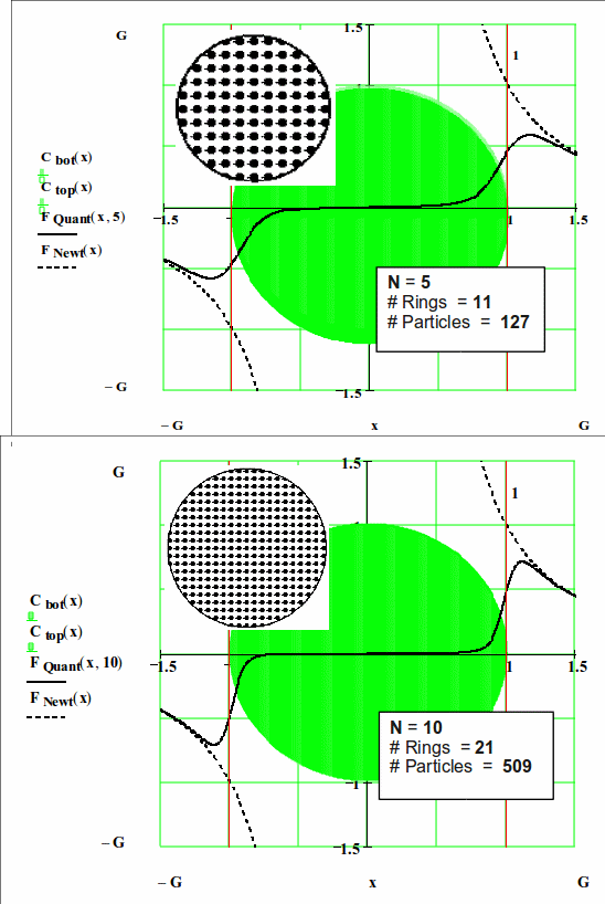
If this sounds familiar, it should. We could use exactly the same summation equation we developed previously for the smooth sphere. Only this time, miraculously, it is no longer an approximation increasing in accuracy as we increase N. Now it is an exact equation, in which ( 2N + 1 ) represents the actual number of rings, and hence the quantization of the mass (or charge) in the x - direction. An N of 5 for instance would correspond to our current example above, giving 11 rings.





An astute reader might raise the following objection: In the original equation we spaced the rings equally along the x-axis using Archimedes’ Theorem. Shouldn’t the rings in this case be spaced equally along the sphere surface? Yes they should, and this can easily be incorporated into our equation, as we show in the following pages.

But in the present case we wouldn’t even need to do this to get an immediate, qualitative and very accurate understanding of what quantization of any kind does to the force in the x-direction. After all, we would like to know about almost any hollow polyhedral molecule. For this purpose we could assign arbitrary masses to each ring, and space them in almost any rough fashion. This would correspond to replacing various atoms in a polyhedral molecule with different elements, or slightly changing the bond angles.

An important point is that we don’t need calculus ( integration ), and in fact it would defeat our purpose, since we want to keep the mass ( or charge ) quantized spatially, not smear the actual gradient of forces into a blurred average of the real picture.


3. Discrete Form of Hollow Sphere Equation




In order to space the rings equally along the surface, we divide the distance into equal parts. For ( 2N + 1) rings, the distance (and angle) in radians is
phi = ( i / N ) * ( pi / 2 ).
We continue our previous strategy of sweeping i from -N to +N. in whole integers. This again allows the sign to automatically handle ring distances, angle directions, force directions, and both small and negative values for the position of the test-mass on the x – axis.

Since there are a lot of variables, the flow chart will help clarify the chain of dependence.


Each variable is related to those below by a simple formula. This allows us to build an overall formula in terms of the loop counter i :


…And we are ready to assemble a summation formula for the quantized sphere.


4. Formula and Graph for Quantized Hollow Sphere

We have plotted a few sample values. ( N = 2 for instance corresponds to a dodecahedron. ) As we increase the # of rings, ( = 2N + 1 ), we can see the curve evolving from that of a single ring toward the shape for a continuum sphere. Even with as many as 41 rings ( # of particles over 2000! ) there remain significant forces inside the sphere. Thus for small numbers of particles ( mass or charge ) the Sphere Theorem is extremely inaccurate, and this is independent of sphere size, applying for instance to room-size objects with small quantities of charge.






5. Sample Hollow Spheres of Discrete Particles












6. Summary and Conclusions with FAQs


We have shown that when mass is 'quantized', that is, localized in particles or discrete packets in space rather than spread out as a continuum over the surface, the Sphere Theorem fails. Forces are not balanced or neutralized at every point inside a hollow sphere. And the net results of the imbalances cause the whole inside volume of the sphere to be unstable, with a net force attracting particles to the nearest surface. The field strength and attraction increases as the inner surface is approached.

Q: 'So what? Gravity is only an approximation at the atomic level. Big deal.'

A: But this is not the actual case at all. Our findings are not based upon absolute sizes or fixed scales in any way. They are simply a result of the clumping of mass, i.e., discrete packeting, or 'quantization' of distribution. While the Sphere Theorem certainly does fail at the molecular level, it also fails at any size where one is dealing with clumping or discreteness with the aspect at hand. This could be mass, or charge, or any other localized object or attribute which induces a force. While the actual 'size' of particles relative to their spacing may be unknown, scattering patterns clearly indicate that both mass and charge are indeed practically 'point-particles' in their effect. The collapse of the Sphere theorem is based not upon sizes, but 'point-like' behaviour.
The error is more closely related to numbers of particles than sizes. For instance, a three-meter aluminium sphere could carry a static charge of only a few hundred electrons. In this case, the Sphere Theorem would be grossly inaccurate, since the point charges would be spread out and the field would be as uneven as a golf-ball, inside and out! Expecting charged particles inside it to drift free is absurd. If anything, with fixed particles, errors will be amplified at larger sizes and distances.
As another example, being near the surface of the earth using the Sphere Theorem as a special case of the Center of Mass theorem would result in an inaccurate measure of the gravity field, and would mislead us as to the true value of the Gravitational Constant (or its universal component).
( That's right: We don't know the real Gravitational Constant at this time: The calculated value is currently only useful as a coordinator of mass to distance units in the vicinity of the earth's surface. There is no theoretical justification to treat it as a universal constant for all sizes and distances. )

Q: What happens when the test particle passes through the surface of the sphere?

A: Under the discrete particle model, the actual surface of the sphere doesn't really exist. It is only a geometrical surface upon which we locate the particles of interest. It could be 'real', in the sense of it being a thin layer of atoms or molecules, as in the three-meter aluminium sphere containing charges. Or we could simply be interested in the gravitational field of the atoms themselves. In either case, the particles of interest are still particles. The chances of actually having a collision or a near-collision with our test-particle would be extremely small, but determined by a typical scattering-matrix. In most instances, the particle would experience the 'softened' and unbalance field we have shown in the text.
Now and then, a particle passing too close to a concentrated point-mass or charge on the surface would experience extremely high forces. Note that even here, those forces would not in any way cause the test-particle to experience a 'balanced' potential field entering the sphere. Instead, the test-particle would be extremely deflected off it's path. It would not proceed straight ahead as predicted by Newton's Sphere theorem.
Our method of approximation is the most accurate and useful model, because we don't attempt to posit extremely rare head-on collisions (or near-collisions) between test-mass and point-mass on the surface itself. For most real trajectories, our equations will reasonably model the general forces experienced by a test particle passing through.
In passing, we have proposed a new and useful significance for discrete models and quantized summations which take them beyond mere approximations of Newton's Sphere Theorem and place them squarely in the practical category of reasonably accurate models for actual expected and observable effects.

Disproving Newton Pt2: (c) Solid Sphere (cont.)

(C) Force for a Solid Sphere




CONTENTS

1. Force for a Uniform Disk
2. Graphing the Force for a Disk
3. Force for a Solid Sphere ( Disk Method )
4. Formula and Graph for Solid Sphere ( Disk Method )
5. Force for a Solid Sphere ( Shell Method )
6. Integral and Graph for Solid Sphere ( Shell Method )
7. Summary of Part 2 so far:





1. Force for a Uniform Disk

The case of a solid thin uniform disk perpendicular to a test-mass is a standard physics problem, but it is usually presented and solved in an inconvenient form. The formula describes a scenario where disk density and distance are held fixed, while the disk radius is varied by adding mass in the form of more outer rings, or else the distance is varied.
Our interest is in what happens when a given mass is spread out into a disk while distance and mass is held constant. We need a form which shows the actual factor diluting Newton’s original formula, as the point-mass is spread out into a thin uniform disk.
Typical Form:





2. Graphing the Force for a Disk

A look at the basic formula shows it isn’t valid for negative values of distance d ( x-coordinate for the test-mass ), because of the ( 1 – cos ) structure. So we have to tweak it a bit by manipulating the sign using the Absolute Value function. …Voila!
The radius is set to r = 1 so that distance units are in radians of the disk.






Note the vertical asymptote at the origin. Physically, the forces should balance there, and the net force should be zero. Again, the mathematics does not perfectly reflect the expected physical situation.



3. Force for a Solid Sphere ( Disk Method )

We can use an approach similar to the hollow sphere, however, this time the mass will vary for each slice. Now, the constant will be disk density. Again as before, r2 is defined using the Pythagorean Theorem, and we can automatically handle near and far slices by using +ve and -ve values for i :







4. Formula and Graph for Solid Sphere ( Disk Method )

The following formula settles around n > 400, at this scale of graph. The original formula is only valid in the domain D > 1 and appears the same as Newton’s 1/ d2 prediction. Manipulating signs with the Absolute Value function extends the formula to values of D < 1 and allows negative x-coordinates for the test-mass as well.







Comments: When -1 < D < 1 , then during the summation, there will always be a point where D = i / N. Here the disk is at the same location as the test-mass, and the force should be zero1 , but our sign patch will have an undefined denominator. With large N, this single disk should have an insignificant mass and can be ignored.
_______________________
6. zero in the x- direction and balanced in the y and z directions, although the physical meaning of this will be discussed later on.


__________________________________________


5. Force for a Solid Sphere ( Shell Method )

For the shell method, we divide the sphere up into concentric hollow spheres or shells, each having a mass proportional to its area. From this perspective, the total mass of the solid sphere is the sum of the masses of each shell. The force from each shell will be weighted by its fraction of the total mass. It is important to maintain consistency in the method of calculating the masses. For this we waive ordinary volume formulas for the sphere and resort to the following formulas:

The shell surface area would normally be 4r 2, but since the 4 in the denominator and numerator of the shell mass formula cancels out, it can be dropped. Integrating the AreaTotal formula gives simply 1/ 3, simplifying further:


We generalize our integrated formula for a hollow sphere to accommodate any radius, and take the constants to the outside:



6. Integral and Graph for Solid Sphere ( Shell Method )

A graph (below) of the formula using the summation is without surprises, converging well at this resolution with N > 400. The integral can also be set up as follows: ( By inspection, there will be a discontinuity at certain values of D and x due to denominator divide-by-zero cases, as with other formulas. )




7. Summary of Part 2 so far:

We have completed our detailed look at the essential mathematical content of the Sphere Theorem ( ST ). We used only simple algebra and trigonometry to allow almost any reader to follow the steps. Integration was only brought in at the end for completeness, to provide simple, exact and labor-saving formulas, although algebraic methods can be used to achieve any desired degree of accuracy.

We remind the reader at this point that contrary to the Centre of Mass Theorem, (CMT) which is conceded to be an ‘approximation’ however ill-defined, the Sphere Theorem ( ST ) is supposed to be an exact theorem, and working in conjunction with electrostatic formulas, is believed to be accurate down to distances of 10 –13 cm.

(See Berkeley Physics Course: Mechanics Vol 1, 2nd Ed. Pg 270 for example.)

We have shown that the hollow sphere formula suffers from a discontinuity, an undefined singularity when the test-mass is at the surface. This exactly parallels the singularity for the disk formula, and also Newton’s original formula for point-masses. By inspection, it is obvious that these anomalies are simply occasional divide-by-zero errors in the formulas, and have no actual physical meaning. For certain values, the formulas are undefined and nonsensical, and are simply invalid.

At least according to classical notions of reality, the force acting on a particle can be zero or unknown, but not ‘undefined’. On this basis, we assume that a test-mass arriving at the centre of the earth doesn’t experience ‘infinite’ gravity but rather a balance of forces resulting in zero net force. Similarly, a test-mass piercing a hollow sphere doesn’t undergo infinite forces in both directions, but more likely experiences a temporary balance of forces, again resulting in an instantaneous force of zero.

It is a common practice to take an otherwise continuous function with only one problem-point and use it for all other values, substituting a value by hand at that point, rather than just discard it. We have no problem with this pragmatic procedure. It serves to remind us however not to take the mathematical formulas too literally, as to their physical truth claims.
It should be clear that the formulas for the solid sphere also have these discontinuities hidden inside them, since they are built out of the hollow sphere and solid disk formulas. This is especially true of the integral and integrated versions of the solid sphere formulas, even though the discontinuities appear to vanish.

The real problems with the integrated versions of the sphere formulas will be shown in the next section. The danger involved in assuming the integrals have the same accuracy and validity as the summation formulas upon which they are based will then become all too apparent.

Disproving Newton Pt2: (b) Hollow Sphere (cont.)

Disproving Newton Pt2: (b) Hollow Sphere (cont.)



Table of Contents
(A) Creating the Tools We Need 4
Introduction: Simplifying the Problem 4
1. Force between a Barbell and a Test-mass 5
2. Getting the Net Force for the Barbell Using the Cosine 6
3. The Equivalent Point Mass is NOT the Geometric Centre 7
4. The Force for a Ring of Negligible Thickness 8
5. Plotting the Force for the Ring 9
(B) The Force for a Hollow Sphere 10
1. Preliminaries for Calculation 10
2. Archimedes’ Theorem 11
3. Defining the Variables 12
4. Integrated Version for Hollow Sphere 14
5. Appendix: Integrating the Hollow Sphere Formula 15
(C) Force for a Solid Sphere 18
1. Force for a Uniform Disk 18
2. Graphing the Force for a Disk 19
3. Force for a Solid Sphere ( Disk Method ) 20
4. Formula and Graph for Solid Sphere ( Disk Method ) 21
5. Force for a Solid Sphere ( Shell Method ) 21
6. Integral and Graph for Solid Sphere ( Shell Method ) 23
7. Summary of Part 2 so far: 24
(D) Failure of Sphere Theorem at Molecular Level 25
1. A Simple Quantization of Mass 25
2. General Method for Discrete Distributions of Mass 26
3. Discrete Form of Hollow Sphere Equation 28
4. Formula and Graph for Quantized Hollow Sphere 30
5. Sample Hollow Spheres of Discrete Particles 31
6. Summary and Conclusions with FAQs 33







(B) The Force for a Hollow Sphere

1. Preliminaries for Calculation
We can get the force that a hollow sphere exerts upon an external test-mass without any calculus at all. All we need is Archimedes’ Theorem, the Pythagorean Theorem, and our formula for a uniform ring. Let’s see how easy it is:

1. For convenience we replace the GmA mB part of the gravitational formulas with a constant, K. Newton’s formula would now just be K / d2.
2. The radius R of the spherewe will set to 1 and so all distances will now be in units of R.
3. The centre-to-centre distance between test-mass and sphere is D, which we leave as a variable but is fixed for any given example. Our formula will be in terms of D, with D in units of R.

The basic idea is simple: We divide the hollow sphere into rings and use our ring formula to get the force from each ring. Then we add them up.







However, two problems pop up:

1. How do we figure out the mass for each ring?
2. How do we figure out the size and distance for each ring?

2. Archimedes’ Theorem
It turns out the mass problem solves itself, if we know Archimedes’ Theorem! Take a sphere and a cylinder with the same diameter. Let two parallel planes cut through them both. Archimedes showed that the surface area of the sections between the planes is the same! But as long as the spacing is fixed, the area between will be the same anywhere on the cylinder, and so the area stays constant for the sphere as well!










That is, rings of equal height, they will automatically have the same area, and mass too. This may seem spooky, but the explanation is simple enough: As the rings’ radius decreases, the tilt of their surface increases just enough to keep the area constant. If the mass is equally spread over the surface, then the area is proportional to mass.




3. Defining the Variables
If we start in the middle and work out toward the edges taking the rings in pairs, each pair will have the same radius, saving some effort.
Ring Mass: Dividing the sphere into 2N rings of equal width ensures that each ring has the same mass. ( via Archimedes’ theorem ) The mass of the whole sphere, mB = 1. This makes the mass of each ring, mi = mB / 2N = 1 / 2N.
( The i subscript identifies each ring for our loop. ) It is true that the curved ‘sphere-slices’ aren’t really rings of negligible thickness, but we can make them as close as we like by increasing the number of slices, 2N.
Coordinates: However, the forces for near and far ring are different, so we have to do each separately. We place the sphere at the origin (0,0), slice the sphere vertically, and use the x-axis for most distances. If i is our counter, and 2N is the number of rings and R = 1 ( the sphere radius ), then we sweep i from – N to + N, and ( i / N )is just the x-coordinate of each ring, which goes from -1 to +1.



Ring Distance: Since the test-mass distance will normally be given as centre-to-centre,5 we define ring distance in those terms.
dnear = D - i / N dfar = D + i / N
Conveniently, our choice of origin and using – and + values for i handles the signs automatically, so the form D - i / N is good for both near and far rings.



Ring Radius: ( via Pythagorean theorem )
When setting up our variables, we might be inclined to define the ring radius, ri in terms of the angle f directly. For instance, ri = sin f, and f = cos-1 ( i / N ).
Rather than insert sin (cos-1 ( i / N ) ) into our formula, we can get ri more simply and directly: Make a standard right triangle around angle f, by using the sphere radius R = 1 as one side and dropping a vertical to the X-axis where the ring will be. ( see diagram. ) The ring radius is then just the y-coordinate. We solve for y using the Pythagorean theorem. y 2 = h 2 - x 2 …h = hypotenuse = 1 )
ri 2= R 2 - ( i / N )2 = 1 - ( i / N )2 ( we won’t need ri itself, just ri 2 …)
So we only use the perspective of the angle f to determine ri 2 in terms of the radius of the sphere. But after that, we are done with it. For the gravity formula we want the perspective of the angle q . But again we can avoid all the trigonometry and angle-juggling by simply working with the distances directly anyway.

Ring Formula:
We also have a choice of forms for the gravity formula for a ring, (see above) but the following version is convenient, substituting in for h via Pythagorean theorem :





Substituting in d and r2 and simplifying the denominator gives the final formula for the hollow sphere: ( note: exponent on r is already handled )



For any given sphere and test-mass at a fixed position, the only variable is i. In fact, the same formula is valid for both inside and outside the hollow sphere, if we allow the (-+) sign to represent the direction of the force along the axis. Good results can be obtained with N > 1000. While this is not practical by hand, it is trivial to write a small computer program to loop the sum and graph the formula. The graph will approximate Newton’s claim regarding the field fora hollow sphere.
We now have a pretty frightening looking formula. But all this is really saying is that we have to integrate our summation formula to make it exact.
Integrating the formula gives us the following simpler formula:

(We show how we integrated this formula below.) And what is this
formula? It is just Newton's original Inverse Square formula with a toggle factor (Absolute Value function) that turns off the force when the test-particle is inside the sphere.
Is it exact? Mathematically yes. Except as always, the formula has discontinuities and is meaningless when the denominators are zero. (the border of the sphere surface). Does it accurately reflect the physical reality inside the sphere?


4. Integrated Version for Hollow Sphere
The Integral form is of course much faster, and more accurate, provided we accept the assumptions which went into it. ( These will be discussed later. )

The steps for the integration have been skipped. Those who can do the calculus won’t need any help to check the result for themselves. The final integral performs as expected by standard theory, so no controversy with Newton can be found (or resolved) along those lines.







Plotting the Force for the Hollow Sphere
Note the finite limits approaching the vertical asymptote ( which is present ) at the surface, shown on the graph. These are two clues that the mathematics is not a perfect representation of the physical situation.* (That is, the formula fails to describe the physical situation when D=R, since dividing by zero is an illegal operation).



__________________________________________

Disproving Newton Pt2: Hollow Sphere Calculation

Disproving Newton Pt2: Hollow Sphere Calculation




Disproving Newton
Part 2



Calculating the Force for a Sphere

By Rogue Physicist, Mastervalver and Metafrizzics
(C) 1999, Updated Aug 24, 2005

Synopsis: Part 2 In this section we derive some tools and give a mathematical treatment of both hollow and solid spheres. Then follows an analysis, which tries to lay bare the assumptions supporting the bridge between the mathematics and the physical reality. In the following section, we show in detail how the Hollow Sphere Theorem breaks down at sizes smaller than about 10,000 times the diameter of an atom. The results also apply to spheres of any size having low numbers of charges, in the range of < 10,000 electrons or holes. This is obviously a significant finding, for which test by experiment is a reasonable expectation.

Table of Contents
(A) Creating the Tools We Need 4
Introduction: Simplifying the Problem 4
1. Force between a Barbell and a Test-mass 5
2. Getting the Net Force for the Barbell Using the Cosine 6
3. The Equivalent Point Mass is NOT the Geometric Centre 7
4. The Force for a Ring of Negligible Thickness 8
5. Plotting the Force for the Ring 9
(B) The Force for a Hollow Sphere 10
1. Preliminaries for Calculation 10
2. Archimedes’ Theorem 11
3. Defining the Variables 12
4. Integrated Version for Hollow Sphere 14
5. Appendix: Integrating the Hollow Sphere Formula 15
(C) Force for a Solid Sphere 18
1. Force for a Uniform Disk 18
2. Graphing the Force for a Disk 19
3. Force for a Solid Sphere ( Disk Method ) 20
4. Formula and Graph for Solid Sphere ( Disk Method ) 21
5. Force for a Solid Sphere ( Shell Method ) 21
6. Integral and Graph for Solid Sphere ( Shell Method ) 23
7. Summary of Part 2 so far: 24
(D) Failure of Sphere Theorem at Molecular Level 25
1. A Simple Quantization of Mass 25
2. General Method for Discrete Distributions of Mass 26
3. Discrete Form of Hollow Sphere Equation 28
4. Formula and Graph for Quantized Hollow Sphere 30
5. Sample Hollow Spheres of Discrete Particles 31
6. Summary and Conclusions with FAQs 33







(A) Creating the Tools We Need

Introduction: Simplifying the Problem
Part of solving any tough task is simplifying the problem any way we can.
Newton's equation for the force looks like this, which seems complicated:



For our purposes we can simplify this equation quite alot before we even start:

1. We can set the radius of the sphere we are going to measure to be '1' . We will measure all other distances in units of this radius. This is important, because the geometric features we'll find are all relative to sphere size.
2. We can set the Gravitational Constant to be '1', by choosing the right units of mass. The Gravitational Constant is not an 'absolute' constant. It really coordinates mass with units of distance, and is set by our choice of units.
3. We can set the mass of each body to be '1' as well. The mass of an object is usually constant. Later we can extend our findings to bodies with different masses and arbitrary sizes.
4. We will centre the Sphere at the Origin of our coordinate axis, so the geometric centre (and centre of mass) will be: (x,y,z) = (0, 0, 0).
5. Our Test-mass will just move along the X-axis. The position of our test-mass will just be the X-coordinate. This will greatly simplify our calculations.

Since G x ma xmb = 1 x 1 x 1 = 1
Newton's equation is now simply the pure Inverse Square Law:

This is the essential and active part of the equation, which says the force falls off according to the distance squared. For now we are going to leave in the 'mass' variables however, to make a few steps in the next section clear.


1. Force between a Barbell and a Test-mass
Take a barbell made of two equal uniform spheres, rigidly connected by a rod of negligible mass, system A. A fixed distance away from the barbell, is another uniform sphere, test-mass B, the same mass as the barbell. 1 It should be obvious that the total force on B is just the sum of the pull from each end of the barbell. We can work out the pull from each end separately, and then just add them. But since each end pulls in a slightly different direction the total force is the vector sumof the forces for A1 and for A2. 2



r is the radius of system A, and d is the basic centre-to-centre distance between the two systems. h is the direct distance to each end, and the angle Theta q shows the actual direction of pull from each end relative to the overall pull, which happens to be toward the geometric centre of system A, due to symmetry.


____________________________________



1. Thegeometric centre (GC) of an object is determined by its shape, i.e., distribution of volume and extension in space. The centre of mass (CM) is determined by the distribution of mass. The CM happens to coincide with the GC in system A , since it is symmetrical in both shape and distribution of mass . These two are not the same as the centre of gravity, which is only relevant in a uniform gravitational field.
Different again is an equivalent point-mass position, which we have to calculate. By equivalent point-mass, (or EPM), we mean a point-mass having the same mass as the system we are replacing. By EPM position, we mean where we must put the EPM to generate exactly the same force as the system. The Sphere Theorem (ST) only claims that the EPM is at the GC for spheres, not barbells or other shapes, so it is natural that we have to calculate it.



2. If we were just solving an example, we could combine the vectors using the parallelogram rule on graph paper, but since we want a general solution for all cases, we want to solve algebraically. This is easily done by using trigonometry.
_____________________________________






2. Getting the Net Force for the Barbell Using the Cosine
Any vector can be split up into a vertical and horizontal component. Here the vertical components for each sphere in system A are opposing and equal so they cancel, leaving only the horizontal components. We can ignore the vertical parts.



Since we really only need the horizontal components, we can write,

Multiplying by the Cosine function correctly scales down the force from each sphere to the net horizontal component only. We then just add these components to get the total force in the X direction.



Substituting the definition of cosine (adj / hyp = d / h), and using Newton,3

These are good given ( h and d ) or ( h and q ). To get it for ( d and q ) we pick a multiplier and combine it in:

What is the physical difference between equation (1.2) and (1.3) ? In terms of h, if we spread the barbell ends apart in an orbit around sphere B, keeping the distance h to each ball constant, the force is proportional to the cosine. But if we keep d constant (the distance between systems) and just lengthen the barbell, the spheres spread apart vertically, and the force drops as the cubeof the cosine!
_________________
3. Note that we use the hypotenuse for the direct distance to each sphere from B, and then get the horizontal component by multiplying by the cosine of the angle from the horizontal.

_____________________

3. The Equivalent Point Mass is NOT the Geometric Centre
The last result is practical, but if we want a version in terms of d and r without having to deal with angles we can take equation (1.1) and do this:

What does it mean? As we shorten the barbell the angle q shrinks, r vanishes, h approaches d, d in the numerator cancels out and we simply get Newton’s formula. If we lengthen the barbell q approaches 90o , 1 the force falls away to nearly zero, even though the GC and CM hold position and the mass also stays constant.
Clearly, when the force is dropping then the EPM must be moving further away, off of the geometric centre and CM. So generally, the centre of mass is not relevant for calculating the force between the two systems.
The key here is that the EPM is simply the viewpoint from sphere B. It is only meaningful in relation to some fixed external position. If we swung sphere B around to the other side, the EPM would also move to the opposite side: A non-spherical object has a different EPM for every possible position around it, and each object will feel a force based upon its own personal viewpoint.
_____________________________________
1 Keep in mind that the angle is not between the two spheres from B , but between the horizontal line ( d ) and each sphere. The angle is always < 90o and the cosine is always positive.
_______________________________________





4. The Force for a Ring of Negligible Thickness
Lets replace the shaft of the barbell with a perpendicular ring around the axis. The spheres can be anywhere on the ring, as long as they are opposite one another. The spheres can be replaced by equivalent point-masses. We can even split each point-mass in half, assign each ¼ the total mass, and spread them out equally around the ring. We can do this without changing the total force, since all the mass remains at the same distance and angle from sphere B. Only the vertical components of the force are affected by rearranging, but these stay balanced and cancel. Although the case is now three-dimensional, the equations remain the same. This process can be continued ad infinitum until the mass is equally spread around the ring in increments as fine as we wish.







The real value of our equations is now apparent. They also define exactly the force of a uniform ring of negligible cross-section perpendicular to sphere B. This is the kind of tool we can use to analyze hollow cylinders, spherical shells, and other related shapes.


5. Plotting the Force for the Ring
We can now plot the force for the ring with a radius of one unit, placed at (0,0,0) on our coordinate axis. The test-particle is simply swept along the x-axis, ( d = x ) and we can plot the results by superimposing the graph and the ring in space.




Summary:
It took a couple of pages, but it was worth it. We have shown that the force weakens as a system’s mass spreads out perpendicularly. We have also shown that the true EPM is not  at the GC but further away.

And we have an elegant and powerful equation for the force of a ring.

No fancy calculus was needed.